18 September 2023
There are many two-dimensional (2D) hydraulic solvers on the market these days, all claiming to produce the best and most accurate flood outputs in the quickest time possible. Yet, not all 2D hydraulic solvers are the same, there are many differences and it is worth being aware of some of the terminology to understand what you're getting when you use a 2D hydraulic solver.
2D Shallow Water Equations
The first thing to think about is what equations are being solved to represent the fluid flow. 2D hydraulic solvers can use a number of different approaches to simulate the physics involved with the movement of water. At the top end are those hydraulic solvers which use the full 2D shallow water equations which are derived by integrating the Reynolds-Averaged Navier Stokes equations over the depth of flow, TUFLOW Classic, TUFLOW HPC and TUFLOW FV (in 2d mode) all use this approach. The terms most relevant for flood modelling include mass conservation and the representation of gravity, friction terms, inertia/momentum and sub-grid turbulence.
Other approaches use a simplification of the 2D shallow water equations where some terms are neglected, resulting in kinematic or diffusive wave approximations or even a simplified 1D representation of flow over a surface. With these approaches, momentum is not conserved and therefore they struggle where inertia effects or rapidly varying flows are present. Therefore, these solvers struggle where there are supercritical flows or hydrodynamic shocks and are unsuitable for modelling dam break scenarios or energetic floodplain inundation.
The 2D shallow water equations can be extended to 3D, such as TUFLOW FV in 3D mode, by using turbulent and scalar mixing models for vertical exchanges which can be useful for 3D hydrodynamics at scale. 3D hydraulic solvers, which simulate the full Navier-Stokes equations, can model more complex 3D hydraulics, which can prove useful when modelling specific structures, but the spatial and temporal scales at which these solvers can simulate in a timely manner make it difficult to apply them to anything larger than the structure scale.
Fixed Grid versus Flexible Mesh Approaches
To undertake the hydraulic calculations, first the underlying topography needs to be discretised. There are typically two main approaches to this, a fixed grid and a flexible mesh. A fixed grid approach uses a grid of uniform cell sizes for the model domain. These are computationally efficient in terms of memory requirements and on a per-cell basis are quicker to simulate than flexible mesh elements. Flexible mesh approaches use a mesh of irregular elements, commonly triangles and quadrilaterals but often more complex shapes, to represent the underlying topography. Flexible mesh approaches have the benefit of being able to be aligned with various geometric shapes, for instance around buildings, but the mesh generation can be time-consuming and there are associated run time overheads. Whereas fixed grids are less geometrically flexible, their computational efficiencies plus control over the smallest cell size, makes them attractive. Approaches such as Quadtree, which allow spatial variation in cell size within a fixed grid scheme as shown in Figure 1, and sub-grid sampling explained later, provide much of the flexibility provided by a flexible mesh scheme whilst maintaining the efficiencies of fixed grids.

Figure 1: Quadtree Mesh Example with Cell Size Variation within a Fixed Grid Scheme.
An often overlooked benefit of a fixed grid scheme is the consistency in post processing differences when comparing results from baseline and option analysis model simulations. The consistency in the underlying grid ensures any differences in outputs are a consequence of the implemented option (e.g. topography changes) rather than any changes in the geometry of the underlying mesh. Conversely, with a flexible mesh, differences may appear in parts of the mesh remote from the area of changes, due to changes in the mesh.
Finite Difference vs Finite Volume vs Finite Element Approaches
There are a number of approaches in which the shallow water equations mentioned in the previous section are discretised and calculated through space. Finite difference methods, such as those used in TUFLOW Classic, employ a regular grid to approximate the partial differentials in an equation by differences between values at nodes spaced a finite distance apart. The fixed set of nodes results in a structured grid.
With a finite volume approach, space is divided into geometric shapes over which the shallow water equations are integrated to give equations in terms of fluxes through the control volume boundaries. By assessing the cell fluxes, a perfect mass and momentum conservativeness occurs as the flux out of one cell is equal to the flux into an adjacent cell. Finite Volume methods can be used upon both structured, like TUFLOW HPC, and unstructured grids, like TUFLOW FV.
Finite element methods use an unstructured grid to describe the area of interest. These regions are partitioned finite nodes where the calculations take place. The finite element approach is conceptually less accessible and generally results in longer run times and therefore aren't commonly seen in commercial 2D solvers.
Implicit vs Explicit Schemes
There are two approaches in which hydraulic solvers undertake the hydraulic calculations through time. Implicit schemes, such as TUFLOW Classic, use values from the previous timestep (n) and the new timestep (n+1). Alternatively, in explicit schemes, it involves values from the previous timestep only. Implicit schemes are of greater accuracy theoretically but require the hydraulic calculations to be carried out for the whole model domain rather than on a node or control volume basis. Traditionally, 2D hydraulic solvers were dominated by implicit finite difference approaches, which were able to utilise larger timesteps and therefore be run in a more efficient manner using the hardware available at the time(ie. single core processors). Although quicker, finite difference solvers are prone to numerical instabilities and are not as easily parallelised using more recently developed computational hardware.
Explicit schemes, such as TUFLOW HPC, are easier to implement and can be distributed more easily across multiple Computer Processing Units (CPU) and/or Graphical Processing Units (GPU) for significant speed gains. The explicit schemes are subject to a timestep limitation such as the Courant-Friedrichs-Lewy condition for stability which, although allowing adaptive timestepping, can result in very small timesteps where very small cell sizes, high depths or high velocities occur. Implicit schemes are not subject to such limitations but are limited in terms of accuracy should the timestep used be too large for adequate solution convergence to occur.
First-Order vs Second-Order Solutions
The solution order refers to the approximation to solve the differential equations required to solve the shallow water equations. A first-order solution scheme uses the simplest form of numerical approximation by commonly using the slope of a function to estimate the value of a function at the next timestep. First-order solution schemes are generally simpler and easier to implement which is why many software companies will market their solvers based on their solver speed. However, the first-order schemes struggle to provide accurate solutions, often generating significant numerical diffusion, particularly during highly transient flows, as are often encountered when modelling floods. In terms of hydraulics, first-order schemes tend to over predict water levels, predict later arrival times and narrower wetting events, and can fail to capture small-scale transients. Second-order solution schemes are more complex to solve, by using two function evaluations at different points within a timestep, which does result in slightly slower simulations however significantly improved accuracy results, especially where complex, transient flow occurs.

Figure 2: Numerical Error as a Consequence of Lower Order Solution Schemes.
The longitudinal water surface profile in Figure 2 provides observed water levels along a length of the Brisbane River during the 2011 floods. TUFLOW HPC was used to replicate the event and subsequently used to demonstrate the difference in outputs as a consequence of the selected solution scheme order, with the simpler first-order solution scheme over-predicting the water levels.
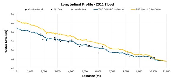
Figure 3: Hydraulic Model Result Comparison Associated with Different Solver Order Assumptions (Brisbane River Longitudinal Water Surface Elevation Profile)
Eddy Viscosity
Turbulence is a fundamental motion in non-laminar flows and affects the velocity and momentum transfer within the flow and is a critical part of the overall energy loss mechanism. Turbulence provides a near-infinite level of detail within fluid flows. It is impractical to model hydrodynamics at a resolution to resolve the eddies that exist within non-laminar flow. For this reason, it is common to represent the presence and effect of eddies using an ‘eddy viscosity’ model.
Many solvers, particularly first-order solution schemes, will neglect the representation of turbulence, instead incorrectly lumping it into numerical diffusion. Whilst these schemes will appear quicker, they will require significant calibration to represent accurate hydrodynamics, typically requiring non-standard Manning’s n resistance values to compensate for the non-physical numerical assumptions. Schemes adopting this approach typically demonstrate increased sensitivity of results to the cell size.
There are numerous approaches to representing the eddy viscosity within a solver, from simple constant approaches to more sophisticated calculation approaches. Where mesh sizes vary within the modelling domain, turbulent parametrisation should be independent of the cell size.
Topographic Representation
Historically, computational hardware and data availability meant that hydraulic model cell size were typically at the same level of resolution as Digital Terrain Models (DTM). As a result, a hydraulic model cell had a single elevation value taken at the centre of the cell which provides a linear relationship between the cell water surface elevation and the potential cell storage volume, which is then used in the hydrodynamic calculations. TUFLOW also takes the elevation at the centre of each cell face for the determination of fluxes between grid cells. Where the cell size reflects the topography within the DTM, this approach is valid. However, with the increased collection of both conventional Light Detection And Radar (LiDAR) and terrestrially-acquired LiDAR at resolutions much higher than the typical hydraulic model cell size, there is a loss of potentially important topographic detail. Sub-Grid Sampling (SGS) seeks to address this issue by sampling the underlying DTM within the hydraulic cell and constructing a non-linear relationship between the cell water surface elevation and the potential cell storage volume. Cell face elevation values can also be sampled. SGS provides a much better representation of the underlying topography compared to the more simplistic single elevation cell centre approach. As a result, SGS exhibits substantially less or negligble result sensitivity to cell size assumptions, and larger cell sizes can be utilised whilst still representing the underlying topography. The two animations in Figure 4 show the same dam breach into a lowland area represented with a 10m cell size. The use of SGS represents the drainage channels more accurately and therefore better represents the flooding of the breach within the drainage channels. The conventional approach of using a single elevation value per cell, coarsely defines the topography, causing an unrealistic blockage in the drainage channels, leading to increased (also unrealistic) inundation of the floodplain.
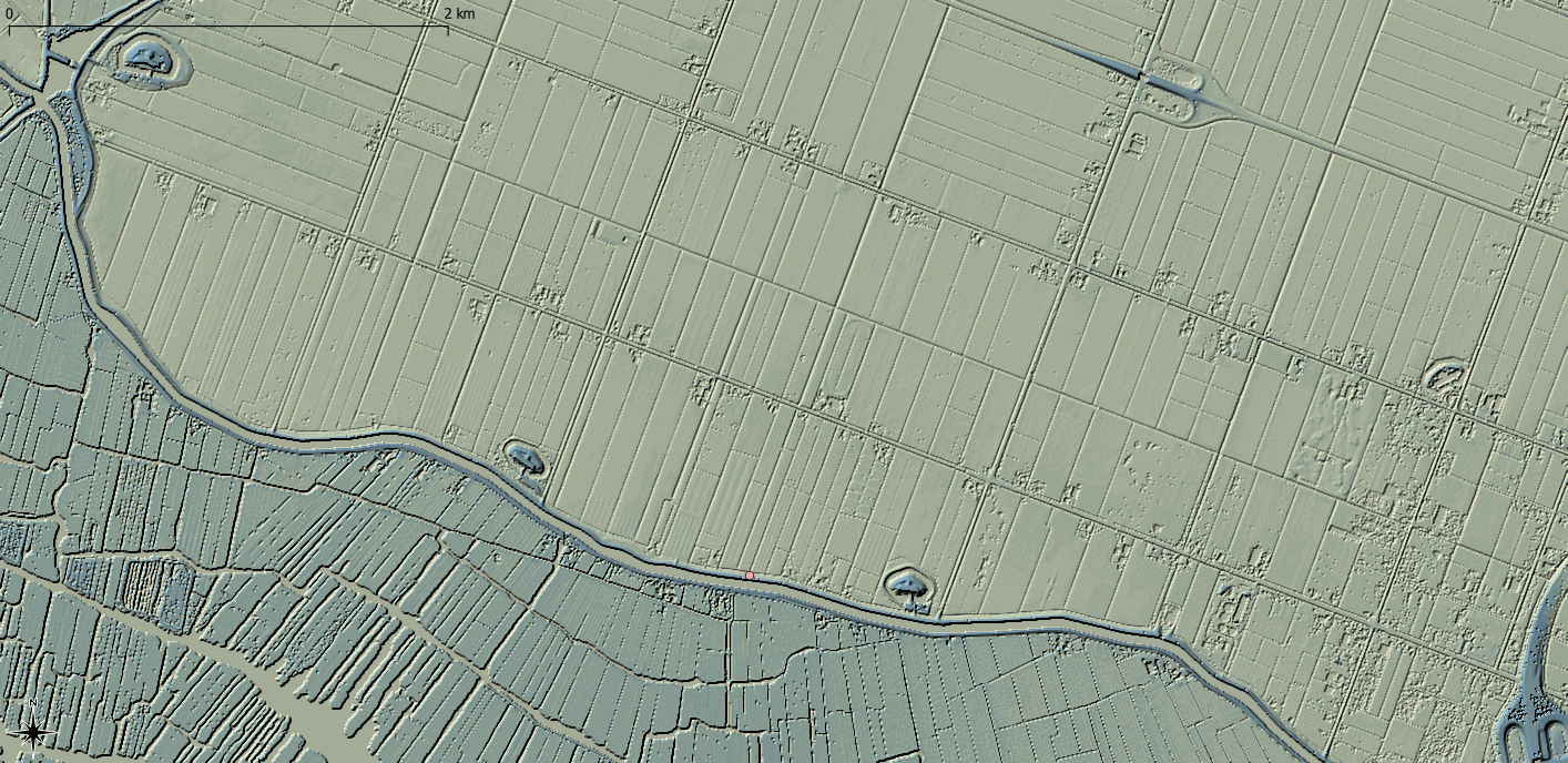

Figure 4: Outputs from a breach modelling exercise using a 10m grid with the upper animation using a traditional one elevation per cell approach and the lower using a Sub-Grid Sampling (SGS) approach (to sample the 1m DTM). Output resolutions are both at 5m resolutions.
In the case of a fixed grid scheme, such as TUFLOW HPC, the sub-grid sampling approach also provides a negligible sensitivity to the grid orientation.
Summary
With the continued development of computational hardware, 2D hydraulic modelling solvers have developed from efficient but complex approaches to a wider range of brute force methods which rely on more simplistic approaches, which can subsequently be carried out more efficiently on more modern computational hardware such as GPU cards. With this has become a plethora of marketing campaigns suggesting that each solver is the quickest and most accurate on the market. However, it’s always worth understanding the different 2D approaches and asking yourself the following questions when considering using a 2D hydraulic solver:
Finally, to truly test the validity of a 2D solver for your project, carry out the following simple checks during your model development phase. These tests should be repeated for each model as the hydraulic complexity and sensitivity to cell size and timestepping varies from model to model.
TUFLOW - Info
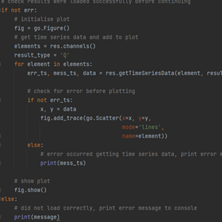
TUFLOW's PyTUFLOW toolbox provides an interface into the TUFLOW results file which allow the user to quickly and consistently process model outputs. An example is provided which integrates PyTUFLOW with the Plotly graphing library to produce interactive plots comparing modelled outputs with observed flow measurements.

TUFLOW - Info
Although there isn't a new TUFLOW release in time for Christmas, that does not mean there aren't any TUFLOW goodies to sink your teeth in to in the New Year.
TUFLOW - Info
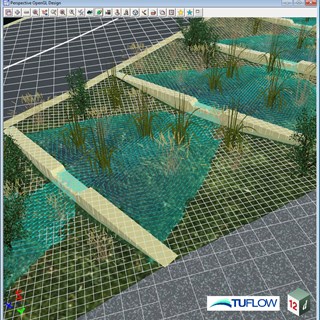
12d Model and TUFLOW provides an excellent way of integrating what were historically siloed areas of responsibility for civil designers, flood modellers and client liaison. This example showcases how 12d Model - TUFLOW can help customers overcome their problems in design and flooding projects by providing the connectivity from concept through to construction.
TUFLOW - Info
The Pix Brook Flood Study is a multi-stakeholder options and feasibility investigation needing an integrated catchment wide model. TUFLOW was chosen due to its ability to represent surface water, fluvial and pipe networks within the one modelling software.