
31 March 2023
Calibrating a water quality model – no matter what modelling package is being used – can sometimes be a daunting task. Why? Because there are many interacting water quality variables (such as dissolved oxygen, organics, phytoplankton and so on) and these variables can in turn have many (also interacting) parameters that control their respective behaviours. As an example, a basic water quality model that simulates common trophic processes up to and including two phytoplankton groups can have more than 10 water quality variables and 150 parameters. So, in the very likely event that a water quality model does not calibrate perfectly the first time it is run, then how do we get the calibration on track, and quickly?...there are simply too many parameters to even know where to start! That’s where the diagnostic variables reported by TUFLOW FV’s Water Quality (WQ) Module come in handy – they help take the guesswork out of water quality modelling.
Let’s investigate the power of the water quality diagnostic variables using a simple oxygen dynamics example. A future Insights article will describe a more complex application involving phytoplankton.
Consider a hypothetical project concerned with oxygen dynamics in a water supply reservoir, and that some of the project deliverables include preparation of design drawings for a new bubble plume destratifier. This destratifier delivers compressed air to a bottom mounted perforated pipe (see Figure 1), and when operating is intended to break down the observed summertime thermocline in the reservoir. This is required because the thermocline isolates bottom (deep) waters from the surface, and so they become anoxic and problematic for downstream water treatment plants when extracted for potable supply. The ultimate intent of the bubble plume is to therefore improve oxygenation and water health at depth.
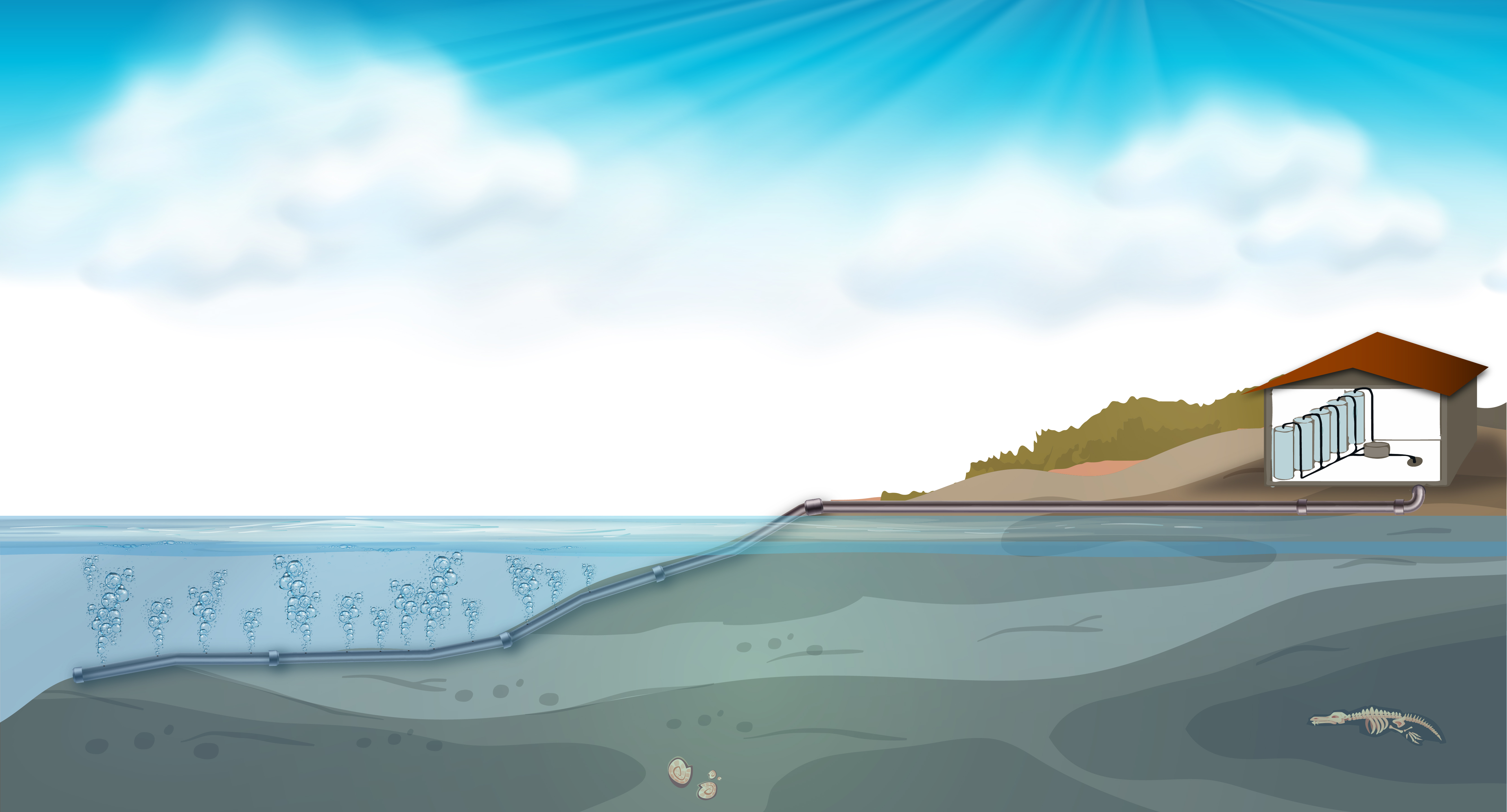
Figure 1: Bubble Plume Destratifier
To design the destratifier, a hydrodynamic and water quality model of the reservoir is to be built to simulate multiannual thermocline development and dismantling, and the associated dissolved oxygen dynamics. Simulations are to include both the existing reservoir (i.e. without a destratifier) and the reservoir under future scenarios with a destratifier installed. These future scenarios are to be used to assist in destratifier design.
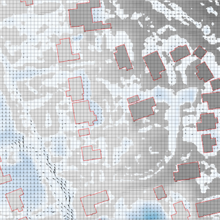
For the purposes of this example, a modified version of the TUFLOW FV water quality tutorial model will be used. A description of the model is available on the TUFLOW FV Wiki. Model files for it can be downloaded from the website. In summary, the tutorial model is an elongated reservoir that receives a single inflow at its upstream boundary and has a single outflow (an offtake for water supply) at its downstream extent. The inflow and offtake are separated by approximately 12 kilometres and the water depth increases closer to the offtake. A plan view schematic of the reservoir is shown below.
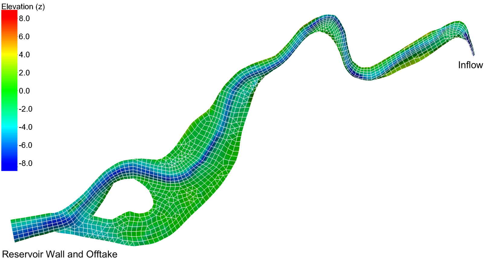
Figure 2: Reservoir Model (Plan View)
Since we are using the TUFLOW FV WQ Module to investigate only dissolved oxygen dynamics, we can deploy the simplest simulation class available within the Module – “DO”. We will also assume that we have benthic chamber measurements of sediment oxygen consumption near the reservoir offtake, and that these have determined that the consumption rate is 3,500 mg of dissolved oxygen (O2) per square meter per day, at 20oC. Applying this rate to the cells near the dam and running the model results in the following quasi-steady state dissolved oxygen concentration profile at the offtake after a week of simulation. Dissolved oxygen profile measurements taken at the same time the simulation completed are also shown.
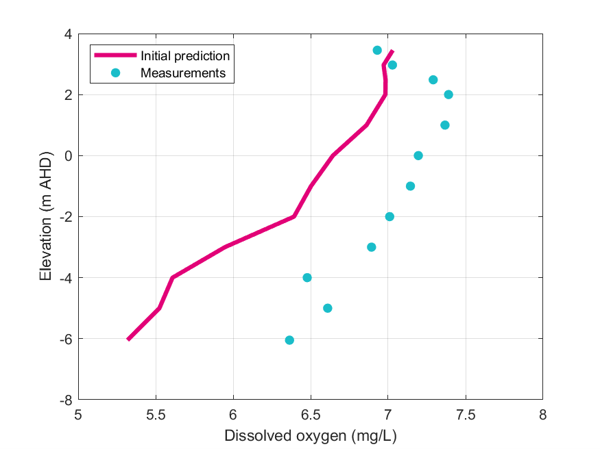
Figure 3: Dissolved Oxygen Concentration Profile (Initial Model Performance)
The figure shows that the modelled and measured dissolved oxygen profiles do not match, and in particular, that the predicted bottom dissolved oxygen concentrations are generally too low. But what to do? Well, we start by interrogating the TUFLOW FV WQ Module diagnostic variables to see what process (of the many available) is controlling oxygen concentrations at depth. We can’t take the (oft used) sledge hammer approach and change the sediment oxygen consumption rate because this is a field measurement that has cost a great deal of money to collect! So, the first thing to do is understand the fluxes of oxygen that control the shape of this concentration profile.
The fluxes of oxygen that control this profile are described in Section 3.1.2 of the interactive online TUFLOW FV WQ Module manual. The relevant figure from the Manual is reproduced below, showing that (in this simple example) atmospheric aeration and sediment consumption of oxygen are the controlling processes.
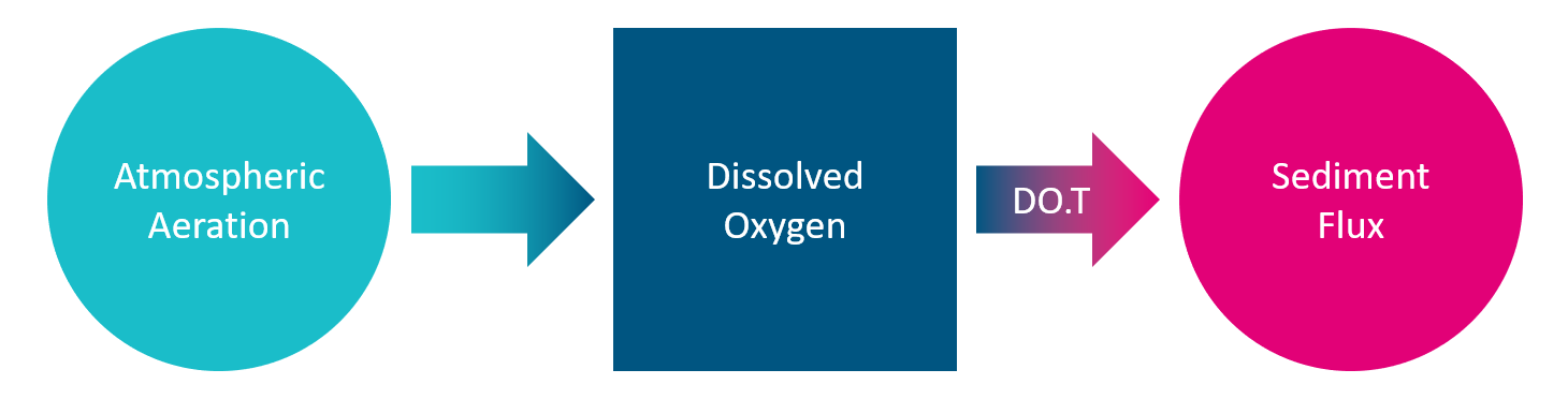
Figure 4: Relevant Dissolved Oxygen Fluxes
By design, both these fluxes are reported by the TUFLOW FV WQ Module as diagnostic variables, for all relevant model cells at all output timesteps. These diagnostics allow us to gauge the relative magnitude of the controlling fluxes at the location of interest, and therefore they provide guidance on which water quality processes to consider reparameterising. These fluxes, at a cell near the reservoir offtake, are plotted below. A positive flux represents delivery of dissolved oxygen to the water column.
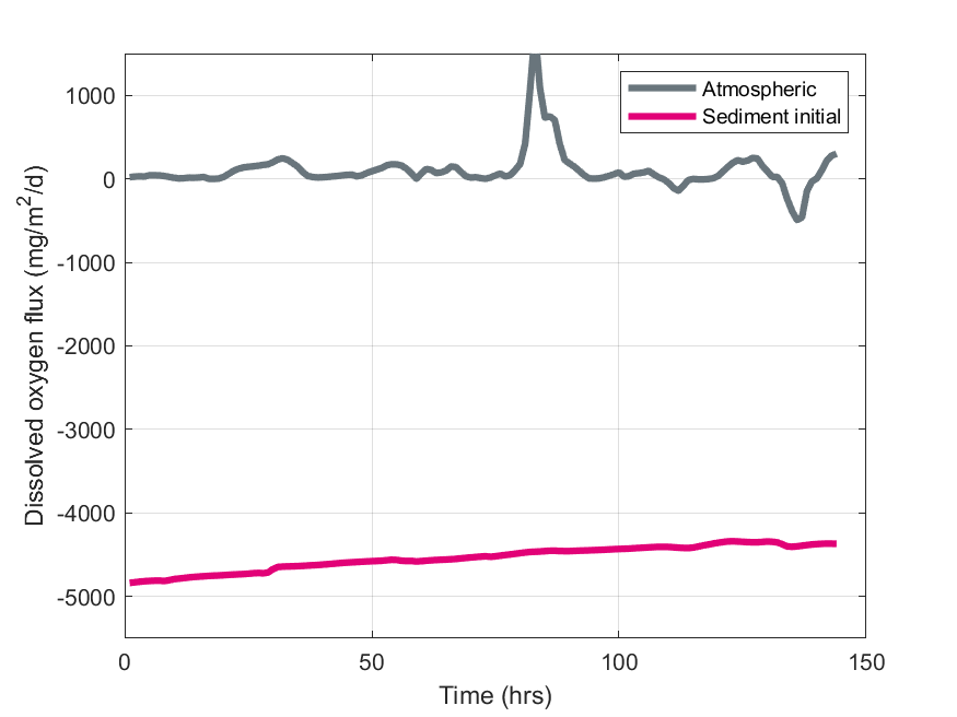
Figure 5: Diagnostic Variables: Initial Oxygen Fluxes
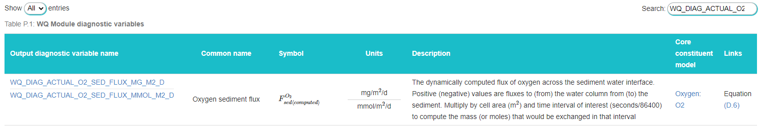
The figure highlights that the sediment consumption of dissolved oxygen is (by far) the flux of greatest magnitude, and therefore (if we feel this is justifiable) deserving of our attention in our recalibration efforts. Given we are not able to alter the applied sediment oxygen demand rate at 20oC (it has been measured), we must consider other parameters that control sediment oxygen consumption, or flux. Using the diagnostic variable name output by the TUFLOW FV WQ Module (WQ_DIAG_ACTUAL_O2_SED_FLUX_MG_M2_D) or the "common name" field (Oxygen sediment flux) as a search term in the TUFLOW FV WQ Module manual Diagnostic Variables Appendix, we are presented with the following description and pointer to the relevant science in the Links column.
Excerpt 1: TUFLOW FV WQ Module Manual Diagnostic Variable Appendix (Sediment Oxygen Flux)
 |
Clicking on Equation (D.6) takes the reader to the relevant section of the manual that describes the science underpinning the TUFLOW FV WQ Module’s sediment oxygen flux calculations. This section is repeated here for ease of reference.
Excerpt 2: TUFLOW FV WQ Module Manual Science (Sediment Oxygen Flux)
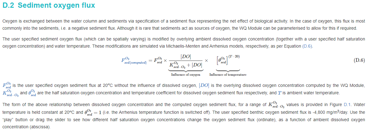 |
The section presents the relevant equation and links to all associated variables. In this case, the half saturation oxygen concentration and temperature coefficient for dissolved oxygen sediment flux calculations are of relevance. The manual also presents an interactive figure that allows the reader to use the slide bar to see the influence varying the half saturation oxygen concentration in Equation (D.6) has on the resultant computed sediment fluxes. Two (non-interactive) snapshots of this figure are presented in a single figure (in pink and blue) below – feel free to try the interactive version in the manual yourself.
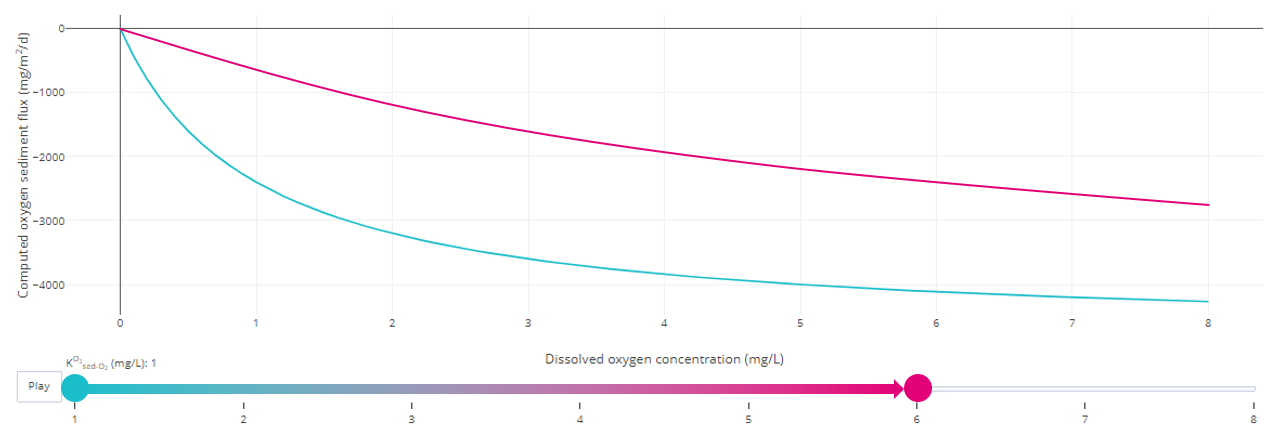
Figure 6: TUFLOW FV WQ Module Manual Interactive Figure Examples
There is some flexibility in adjusting the half saturation oxygen concentration (rather than the measured flux at 20oC), and the manual’s interactive feature tells us that increasing its value decreases the computed sediment flux. Together, therefore, the diagnostic variable and interactive manual suggest that raising the specified half saturation oxygen concentration for sediment oxygen demand may reduce sediment fluxes and increase remaining dissolved oxygen concentrations in the water column – which recalling Figure 3 is our goal.
Applying this change – increasing the half saturation oxygen concentration from 0.5 mg/L to 4.0 mg/L – and rerunning the model in an otherwise unchanged state produces the following oxygen fluxes. The following figure is a repeat of Figure 5, with the initial (pink) and revised (light blue) computed sediment fluxes of oxygen. Atmospheric fluxes are essentially unchanged between models.
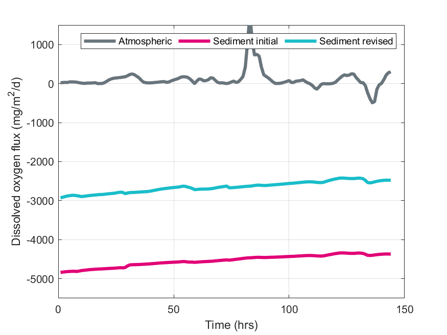
Figure 7: Diagnostic Variables: Revised Oxygen Fluxes
The figure shows that, as determined using the diagnostic variables and supporting science, reparameterisation of the sediment oxygen demand calculations has indeed reduced the magnitude of the computed flux at the location of interest. The revised calculated fluxes are approximately 60% of the original, as intended. The corresponding water column dissolved oxygen concentration profile is presented in blue below. This profile is taken at the same location and time as the profile presented in Figure 3. The dissolved oxygen concentration profile estimate from our initial assessment (prior to the half saturation oxygen concentration reparameterization) is also shown in pink for ease of comparison.
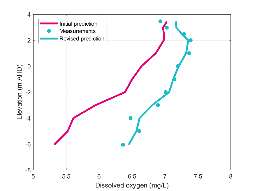
Figure 8: Dissolved Oxygen Concentration Profile (Revised Model Performance)
The figure shows a improved fit to measurements, and our calibration process is well underway almost immediately! The model is now in a good position to be used in designing a bubble plume destratification device.
Using TUFLOW FV’s bubble plume routines in a series of exploratory simulations that built on the calibrated dissolved oxygen model, a suitable bubble design was able to be arrived at. The predicted dissolved oxygen concentration profile (under the influence of the operating bubble plume) at the same location and time as profiles previously shown in this article is presented in Figure 10. The figure shows increased dissolved oxygen concentrations at depth (dark blue line), as intended.
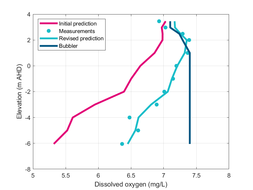
Figure 9 Dissolved Oxygen Concentration Profile (Bubble Plume Destratifier)
In summary, a rapid calibration process for dissolved oxygen has been facilitated through efficient and judicious use of the TUFLOW FV WQ Module’s diagnostic variables, in conjunction with the resources available in the TUFLOW FV WQ Module manual. These sorts of techniques should be adopted by all water quality modellers. Use of diagnostic variables takes much of the guesswork out of calibrating water quality models!
This Insights article is Part 1 of a two part series focusing on water quality model calibration. If you found this article interesting and useful, watch this space for the upcoming publication of Part 2. Part 2 introduces a more complex modelling scenario, considering phytoplankton dynamics in the water supply reservoir.
TUFLOW - Info
Sub-Grid Sampling opens up the door to offer major benefits to Urban Surface Water Modelling, particularly with regards the simulation of property flood depths, an important metric for flood risk management

TUFLOW - Info
Version control is an important part of any model build process. This article highlights the use of the Kart tool to provide an alternative to the traditional approach to spatial data version control within TUFLOW models, bringing with it some exciting features for reviewing changes.
TUFLOW - Info
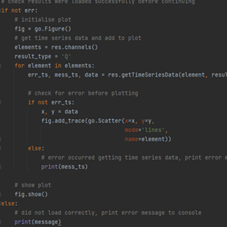
TUFLOW's PyTUFLOW toolbox provides an interface into the TUFLOW results file which allow the user to quickly and consistently process model outputs. An example is provided which integrates PyTUFLOW with the Plotly graphing library to produce interactive plots comparing modelled outputs with observed flow measurements.

TUFLOW - Info
This insights article and associated presentation outlines various tips how to increase your TUFLOW HPC simulation speed.